Técnicas de IA para Biologia

6 - Representation Learning

André Lamúrias

Representation Learning

Motivation

Features are very important

Example: long division using Arabic or Roman numerals
In machine learning, the right representation makes all the difference
Deep learning can be seen as stacked feature extractors, until the final classification

The top layer could even be replaced by another type of model, in theory

Representation learning

Supervised learning with limited data can lead to overfitting
But learning the best representation can be done with unlabelled data

Unsupervised and semi-supervised learning can help find the right features

Motivation

"Meta-priors": what makes a good representation?

Representation Learning; Bengio, Courville, Vincent, 2013

Manifolds:

Actual data is distributed in a subspace of all possible feature value combinations

Disentanglement:

Data is generated by combination of independent factors (e.g. shape, color, lighting, ...)

Hierarchical organization of explanatory factors:

Concepts that explain reality can be composed of more elementar concepts (e.g. edges, shapes, patterns)

Semi-supervised learning:

Unlabelled data is more numerous and can be used to learn structure

Motivation

"Meta-priors": what makes a good representation?

Representation Learning; Bengio, Courville, Vincent, 2013

Shared factors:

Important features for one problem may also be important for other problems (e.g. image recognition)

Sparsity:

Each example may contain only some of the relevant factors (ears, tail, legs, wings, feet)

Smoothness:

The function we are learning outputs similar $y$ for similar $x$

Motivation

"Meta-priors": what makes a good representation?

Representation Learning; Bengio, Courville, Vincent, 2013

If we can capture these regularities, we can extract useful features from our data
These features can be reused in different problems, even with different data

Representation Learning

Unsupervised Pretraining

Greedy layer-wise unsupervised pretraining

Greedy: optimizes each part independently
Layer-wise: pretraining is done one layer at a time

E.g. train autoencoder, discard decoder, use encoding as input for next layer (another autoencoder)

Unsupervised: each layer is trained without supervision (e.g. autoencoder)
Pretraining: the goal is to initialize the network

It is followed by fine-tuning with backpropagation
Or by training of a classifier "on top" of the pretrained layers

Unsupervised Pretraining

Why should this work?

Initialization has regularizing effect

Initially thought as a way to find different local minima, but this does not seem to be the case (ANN do not generally stop at minima)
It may be that pretraining allows the network to reach a different region of the parameter space

Unsupervised Pretraining

When does it work?

Poor initial representations

E.g. word embedding from one-hot vectors

One-hot vectors are all equidistant, which is bad for learning
Unsupervised pretraining helps find representations that are more useful

Example: (Large) Language Models

Known as self-supervised learning, latent representations are called word embeddings

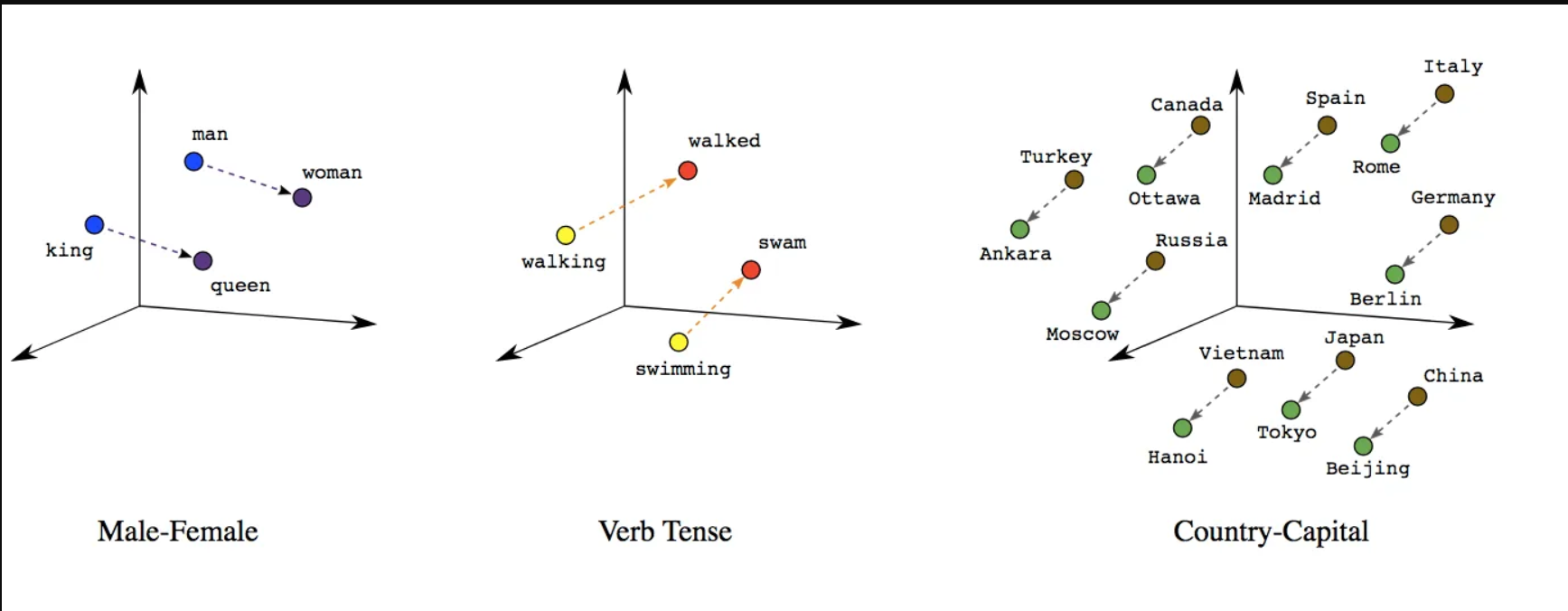
https://developers.google.com/machine-learning/crash-course/embeddings/translating-to-a-lower-dimensional-space

Unsupervised Pretraining

When does it work?

Poor initial representations

E.g. word embedding from one-hot vectors

One-hot vectors are all equidistant, which is bad for learning
Unsupervised pretraining helps find representations that are more useful

Regularization, for few labelled examples

If labelled data is scarce, there is greater need for regularization and unsupervised pretraining can use unlabelled data for this

Example: Training trajectories with and without pretraining

Concatenate vector of outputs for all test set at different iterations

(50 nertworks with and without pretraining)

Project into 2D (tSNE and ISOMAP)

Unsupervised Pretraining

Regularizing effect

Ehrlan et. al. 2010: output vectors for all data, reduce dimensionality, plot

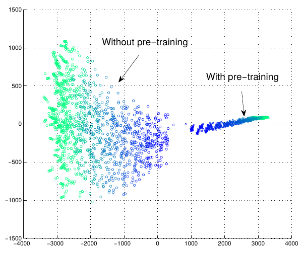
t-Distributed Stochastic Neighbor Embedding and ISOMAP

Unsupervised Pretraining

Unsupervised pretraining is historically important

It was the first practical method for training deep networks
Most DL problems habed abandoned it because of ReLU and dropout, which allows efficient supervised training and regularization of the whole network

For very small datasets, other methods outperform neural networks

e.g. Bayesian methods

Another disadvantage: having two training stages makes it harder to adjust Hyperparameters
Commonly used in some applications, such as natural language processing

Unsupervised pretraining with billions of examples to learn good word representations

Representation Learning

Transfer Learning

Two different tasks with shared relevant factors

Shared lower level features:

E.g. distinguish between cats and dogs, or between horses and donkeys

The low level features are mostly the same, only the higher level classification layers need to change

Shared higher level representations:

E.g. speech recognition
The high level generation of sentences is the same for different speakers
However, the low level feature extraction may need to be tailored to each speaker

Domain adaptation

Same underlying function but different domains

We want to model the same mapping from input to output, but are using different sets of examples
E.g. sentiment analysis

Model was trained on customer reviews for movies and songs
Now we need to do the same for electronics
There should be only one mapping from words to happy or unhappy, but we are training on different sets with different words
This is one example where unsupervised training (DAE - denoising autoencoders) can help

Concept Drift

Similar to Transfer learning or domain adaptation

But occurs when the change is gradual over time

E.g. as the brand becomes more popular, customer base changes from specialized to general

Transfer Learning

Use previous experience in new conditions

The common idea is that we can use what was learned before to help learn now
Extreme examples: one-shot learning and zero-shot learning
Zero-shot learning: no labelled examples of new classes are necessary

Everything was learned on other classes or unsupervised

One-shot learning: use only one labelled example to learn new dataset

The rest was learned on other data

Transfer Learning

Zero-shot learning, example:

Unsupervised learning of word manifold, supervised mapping of known images
A new image is mapped to word manifold

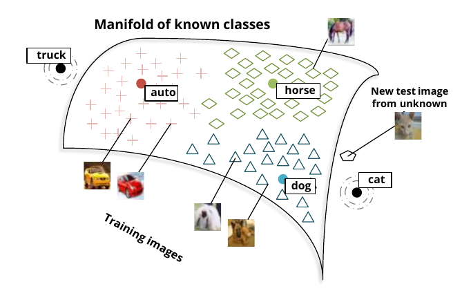
Socher et. al. Zero-Shot Learning Through Cross-Modal Transfer (2013)

Representation learning

Summary

Representation learning

Summary

Improve learning from poor representations

Find the best features

Regularization or feature extraction with unlabelled data
Historically important in deep learning

Still used in NLP (self-supervised learning)

Transfer learning (often supervised)

Representation Learning

Exercise 1: transfer learning
Fashion MNIST to MNIST

Exercise

Transfer learning

Use network trained on Fashion MNIST

Exercise

Transfer learning

Use network trained on Fashion MNIST

Use Keras functional API and pre-trained model

Exercise

Transfer learning

Using pre-trained model:

Create same graph as model we trained last week
Load weights from last week's trained model
Fix weights of convolutional part (won't be retrained)
Recreate the dense classifier and train it on MNIST

Exercise

Prepare dataset

Same process as last week, but with MNIST instead of Fashion MNIST


from tensorflow import keras
from tensorflow.keras.optimizers import SGD
from tensorflow.keras.models import Model
from tensorflow.keras.layers import Input, BatchNormalization, Conv2D, Dense
from tensorflow.keras.layers import MaxPooling2D, Activation, Flatten, Dropout

((trainX, trainY), (testX, testY)) = keras.datasets.mnist.load_data()
trainX = trainX.reshape((trainX.shape[0], 28, 28, 1))
testX = testX.reshape((testX.shape[0], 28, 28, 1))
trainX = trainX.astype("float32") / 255.0
testX = testX.astype("float32") / 255.0

Exercise

Keras functional API

Layer objects are callable (implement __call__ method)
Receive tensors as arguments, return tensors
Input instantiates a Keras tensor (shaped like the data)
Naming layers helps finding them again in the model

We start by recreating the original model architecture


inputs = Input(shape=(28,28,1),name='inputs')
layer = Conv2D(32, (3, 3), padding="same", input_shape=(28,28,1))(inputs)
layer = Activation("relu")(layer)
layer = BatchNormalization(axis=-1)(layer)
layer = Conv2D(32, (3, 3), padding="same")(layer)
layer = Activation("relu")(layer)
layer = BatchNormalization(axis=-1)(layer)
layer = MaxPooling2D(pool_size=(2, 2))(layer)
layer = Dropout(0.25)(layer)
...

Exercise

Chain layers as in the original model
Create the old model and compile it
Load previous weights and disable training in the old model
Note: Flatten layer named for use in new model


...
features = Flatten(name='features')(layer)
layer = Dense(512)(features)
layer = Activation("relu")(layer)
layer = BatchNormalization()(layer)
layer = Dropout(0.5)(layer)
layer = Dense(10)(layer)
layer = Activation("softmax")(layer)

old_model = Model(inputs = inputs, outputs = layer)
old_model.compile(optimizer=SGD(), loss='mse')
old_model.load_weights('fashion_model')
for layer in old_model.layers:
    layer.trainable = False

Exercise

Create new dense layers for new model

The input for this layer is the "features" layer in old model

Then create the new model with:

Old model inputs as input
New softmax layer as output

This chains old CNN to new dense layer


layer = Dense(512)(old_model.get_layer('features').output)
layer = Activation("relu")(layer)
layer = BatchNormalization()(layer)
layer = Dropout(0.5)(layer)
layer = Dense(10)(layer)
layer = Activation("softmax")(layer)
model = Model(inputs = old_model.get_layer('inputs').output, outputs = layer)

Exercise

Now train


NUM_EPOCHS = 5
BS=512
opt = SGD(lr=1e-2, momentum=0.9)
model.compile(loss="categorical_crossentropy",
              optimizer=opt, metrics=["accuracy"])
model.summary()
H = model.fit(trainX, trainY,validation_data=(testX, testY),
             batch_size=BS, epochs=NUM_EPOCHS)

Summary:

Total params: 1,679,082
Trainable params: 1,612,298
Non-trainable params: 66,784

Compare with training all model from the start

Representation learning

Exercise 2: dimension reduction with autoencoder

Autoencoder

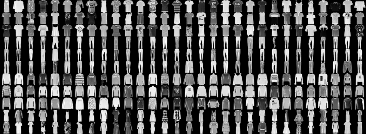
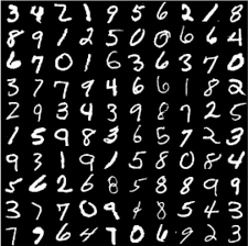
Project MNIST data set into 2D

Autoencoder

Need some extra layers:


from tensorflow.keras.layers import UpSampling2D,Reshape

Encoder:


def autoencoder():
  inputs = Input(shape=(28,28,1),name='inputs')
  layer = Conv2D(32, (3, 3), padding="same", input_shape=(28,28,1))(inputs)
  layer = Activation("relu")(layer)
  layer = BatchNormalization(axis=-1)(layer)
  #[...] parts missing here!
  layer = MaxPooling2D(pool_size=(2, 2))(layer)
  #[...] parts missing here!
  layer = Conv2D(8, (3, 3), padding="same")(layer)
  layer = Activation("relu")(layer)
  layer = BatchNormalization(axis=-1)(layer)

  layer = Flatten()(layer)
  features = Dense(2,name='features')(layer)

Autoencoder

Decoder:


 layer = BatchNormalization()(features)
 layer = Dense(8*7*7,activation="relu")(features)
 layer = Reshape((7,7,8))(layer)
 layer = Conv2D(8, (3, 3), padding="same")(layer)
 layer = Activation("relu")(layer)
 layer = BatchNormalization(axis=-1)(layer)
 layer = Conv2D(16, (3, 3), padding="same")(layer)
 layer = Activation("relu")(layer)
 layer = BatchNormalization(axis=-1)(layer)
 layer = UpSampling2D(size=(2,2))(layer)
 [...]
 layer = Conv2D(32, (3, 3), padding="same")(layer)
 layer = Activation("relu")(layer)
 layer = BatchNormalization(axis=-1)(layer)
 layer = Conv2D(1, (3, 3), padding="same")(layer)
 layer = Activation("sigmoid")(layer)
 autoencoder = Model(inputs = inputs, outputs = layer)
 encoder = Model(inputs=inputs,outputs=features)
 return autoencoder,encoder

Autoencoder

Suggestions

Architecture:

Convolution layer with 32 filters, followed by pooling
Convolution layer with 32 filters, then convolution layer with 16 filters, then pooling
Convolution layer with 16 filters, then convolution layer with 8 filters, then pooling
Dense layer with 2 neurons and linear output, then dense layer with 8*7*7 neurons (relu) and reshape
Convolutions in reverse (8, 16, 16, 32 and 32 filters), and upsampling
A final convolution of 1 filter for the (sigmoid) output.

Training: takes some time (40 epochs or more...)

Details weigh little on the loss function

Save weights after training!

Autoencoder

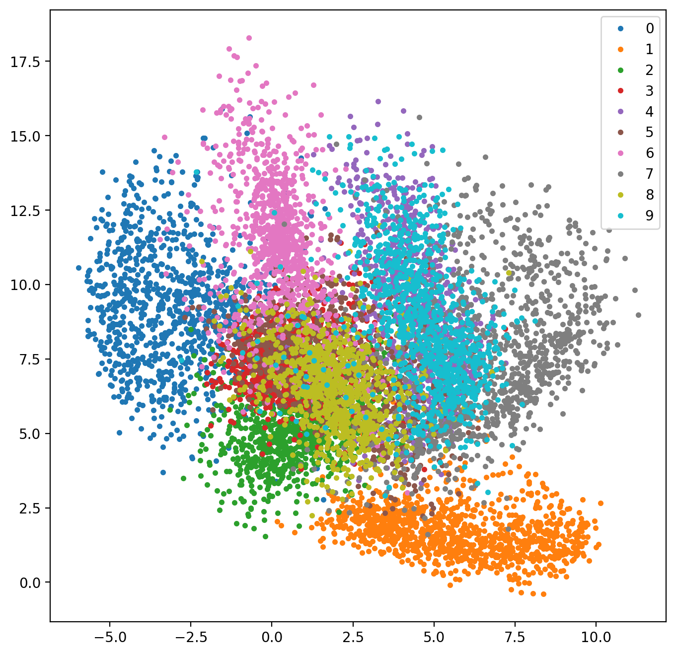
Check representation, plot in 2D:


def plot_representation():
    ae,enc = autoencoder()
    ae.load_weights('mnist_autoencoder.h5')
    encoding = enc.predict(testX)
    plt.figure(figsize=(8,8))
    for cl in np.unique(testY):
        mask = testY == cl
        plt.plot(encoding[mask,0],encoding[mask,1],'.',label=str(cl))
    plt.legend()

Autoencoder

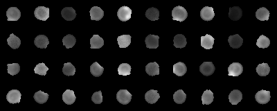
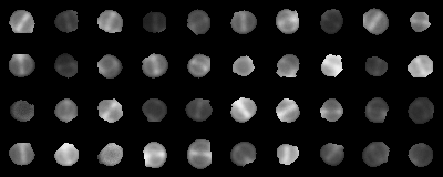
Check reconstruction:


from skimage.io import imsave

def check_images():
    ae,enc = autoencoder()
    ae.load_weights('mnist_autoencoder.h5')
    imgs = ae.predict(testX[:10])
    for ix in range(10):
        imsave(f'T03_{ix}_original.png',testX[ix])
        imsave(f'T03_{ix}_restored.png',imgs[ix])

Autoencoder

Representation Learning

Assignment 1

Context: image classification

Super-resolution fluorescence microscopy images of bacteria
Stage 0: before division starts

Assignment 1

Context: image classification

Super-resolution fluorescence microscopy images of bacteria
Stage 1: septum starts to form

Assignment 1

Context: image classification

Super-resolution fluorescence microscopy images of bacteria
Stage 2: septum is formed, before cell splits

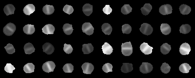
Assignment 1

Data:400 labelled images, 3892 unlabelled images

(40x40 pixels, grayscale)


data = np.load('data.npz')
X_u = data['unlabelled'].astype("float32") / 255.0
X_l = data['labelled'].astype("float32") / 255.0
Y_l = keras.utils.to_categorical(data['labels'],3)

Tasks: experiment, justify and discuss architectures for

A classifier using the 400 labelled images (300 train, 100 validation)
An autoencoder with 3892 unlabelled images (use the 400 for validation)
A simpler classifier using the encoded representations of the 400 labelled images (300 train, 100 validation)

Similar to the exercises we have done so far.
Deadline: March 29 (ideally)

Técnicas de IA para Biologia

6 - Representation Learning

André Lamúrias

Representation Learning

Motivation

Motivation

Features are very important

Representation learning

Motivation

"Meta-priors": what makes a good representation?

Motivation

"Meta-priors": what makes a good representation?

Motivation

"Meta-priors": what makes a good representation?

Representation Learning

Unsupervised Pretraining

Unsupervised Pretraining

Greedy layer-wise unsupervised pretraining

Unsupervised Pretraining

Why should this work?

Unsupervised Pretraining

When does it work?

Unsupervised Pretraining

When does it work?

Unsupervised Pretraining

Unsupervised Pretraining

Unsupervised pretraining is historically important

Representation Learning

Transfer Learning

Transfer Learning

Two different tasks with shared relevant factors

Domain adaptation

Same underlying function but different domains

Concept Drift

Similar to Transfer learning or domain adaptation

Transfer Learning

Use previous experience in new conditions

Transfer Learning

Representation learning

Summary

Representation learning

Summary

Further reading

Representation Learning

Exercise 1: transfer learningFashion MNIST to MNIST

Exercise

Transfer learning

Exercise

Transfer learning

Exercise

Transfer learning

Exercise

Exercise

Exercise

Exercise

Exercise

Representation learning

Exercise 2: dimension reduction with autoencoder

Autoencoder

Autoencoder

Autoencoder

Autoencoder

Suggestions

Autoencoder

Autoencoder

Autoencoder

Autoencoder

Representation Learning

Assignment 1

Assignment 1

Context: image classification

Assignment 1

Context: image classification

Assignment 1

Context: image classification

Assignment 1

Exercise 1: transfer learning
Fashion MNIST to MNIST