Técnicas de IA para Biologia

3 - Activation, Loss and Optimization

André Lamúrias

Introduction

Summary

The vanishing gradients problem
ReLU to the rescue
Different activations: when and how
Loss functions
Optimizers
Overfitting and model selection
Regularization methods in ANN

Activation, Loss and Optimization

Vanishing gradients

Backpropagation in Activation and Loss

Output neuron $n$ of layer $k$ receives input from $m$ from layer $i$ through weight $j$
For a weight $m$ on hidden layer $i$, we must propagate the output error backwards from all neurons ahead
If $\delta s$ is small (vanishing gradient) backpropagation becomes ineffective as we increase depth
This happens with sigmoid activation (or similar, such as TanH)

Vanishing gradients

Single hidden layer, sigmoid, works fine here

Vanishing gradients

Single hidden layer, sigmoid, doesn't work here with 8 neurons

Vanishing gradients

Increasing depth does not seem to help

Vanishing gradients

Increasing depth does not seem to help

Vanishing gradients

Increasing depth does not seem to help
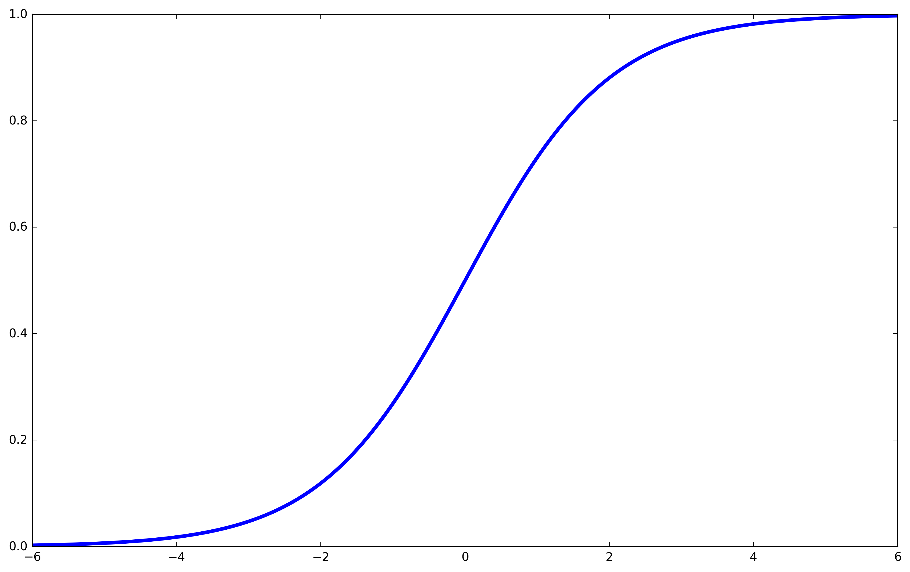
Sigmoid activation saturates and gradients vanish with large coefs.

Activation, Loss and Optimization

Rectified Linear Unit

ReLU

Rectified Linear Unit (ReLU)

Sigmoid activation units saturate

$$y_i = \frac{1}{1+e^{-x_i}}$$

ReLU

Rectified Linear Unit (ReLU)

The same happens with hyperbolic tangent

$$y_i = \frac{e^x - e^{-x}}{e^x + e^{-x}}$$

ReLU

Rectified Linear Unit (ReLU)

Rectified linear units do not have this problem

$$y_i= \left\{ \begin{array}{ll} x_i & x_i \gt 0 \\ 0 & x_i \leq 0 \\ \end{array} \right.$$

ReLU

Sigmoid activation, 3 layers

ReLU

ReLU activation, 3 layers

ReLU

ReLU activation, 4 layers

ReLU

Rectified Linear Unit (ReLU)

Advantages of ReLU activation:

Fast to compute
Does not saturate for positive values, and gradient is always 1

Disadvantage:

ReLU units can "die" if training makes their weights very negative
The unit will output 0 and the gradient will become 0, so it will not "revive"

There are variants that try to fix this problem

ReLU

(Some) ReLU variants

Simple ReLU can die if coefficients are negative

$$y_i= \left\{ \begin{array}{ll} x_i & x_i \gt 0 \\ 0 & x_i \leq 0 \\ \end{array} \right.$$

ReLU

ReLU variant: Leaky ReLU

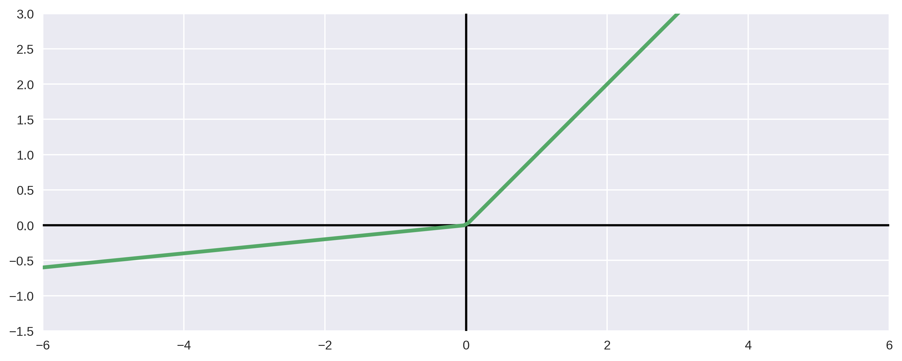
Leaky ReLU gradient is never 0

$$y_i= \left\{ \begin{array}{ll} x_i & x \gt 0 \\ \frac{x_i}{a_i} & x_i \leq 0 \\ \end{array} \right.$$

ReLU

ReLU variant: Leaky ReLU

Note: in Tensorflow

$$y_i= \left\{ \begin{array}{ll} x_i & x \gt 0 \\ a_i x_i & x_i \leq 0 \\ \end{array} \right.$$

ReLU

ReLU variant: Parametric ReLU

Same as leaky, but $a_i$ is also learned

$$y_i= \left\{ \begin{array}{ll} x_i & x \gt 0 \\ \frac{x_i}{a_i} & x_i \leq 0 \\ \end{array} \right.$$

ReLU

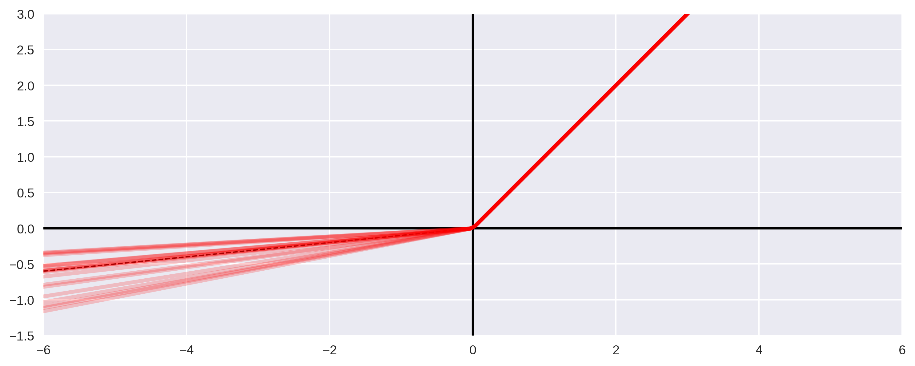
ReLU variant: Randomized Leaky ReLU

Similar, but $a_i \sim U(l,u)$ (average of $l,u$ in test)

$$y_i= \left\{ \begin{array}{ll} x_i & x \gt 0 \\ a_i x_i & x_i \leq 0 \\ \end{array} \right.$$

ReLU

Comparing ReLU variants

Empirical Evaluation of Rectified Activations in Convolution Network (Xu et. al. 2015)

Compared on 2 data sets

CIFAR-10: 60000 32x32 color images in 10 classes of 6000 each
CIFAR-100: 60000 32x32 color images in 100 classes of 600 each

CReLU

Concatenated ReLU combine two ReLU for $x$ and $-x$

Shang et. al., Understanding and Improving CNN via CReLUs, 2016

ELU

Exponential Linear Unit

Exponential in negative part

$$y_i= \left\{ \begin{array}{ll} x_i & x_i \gt 0 \\ a(e^{x_i}-1) & x_i \leq 0 \\ \end{array} \right.$$

Clevert et. al. Fast and Accurate Deep Network Learning by ELUs, 2015

Activation, Loss and Optimization

Activations: which, when, why?

Choosing activations

Hidden layer activations

Hidden layers perform nonlinear transformations

Without nonlinear activation functions, all layers would just amount to a single linear transformation

Activation functions should be fast to compute
Activation functions should avoid vanishing gradients
This is why ReLU (esp. leaky variants) are the recommended choice for hidden layers

Except for specific applications.

E.g. LSTM, Long short-term memory recurrent networks

Choosing activations

Output layer activations

Output layers are a different case.

Choice depends on what we want the model to do

For regression, output should generally be linear

We do not want bounded values and there is little need for nonlinearity in the last layer

For binary classification, sigmoid is a good choice

The output value $[0,1]$ is useful as a representation of the probability of $C_1$, like in logistic regression

Sigmoid is also good for multilabel classification

One example may fit with several labels at the same time
Use one sigmoid output per label

Choosing activations

Output layer activations

For multiclass classification, use softmax:

Note: multiclass means each example fits only one of several classes

Softmax returns a vector where $\sigma_j \in [0,1]$ and $\sum\limits_{k=1}^K \sigma_k = 1$
This can fit a probability of example belonging to each class $C_j$
Softmax is a generalization of the logistic function

It combines the activations of several neurons

Activation, Loss and Optimization

Loss and likelihood

Likelihood

Basic concepts

We have a set of labelled data
We want to approximate some function $F(X) : X \rightarrow Y$ by fitting our parameters
Given some training set, what are the best parameter values?

Simple example, linear regression

$$y = \theta_1 x_1 + \theta_2 x_2 + ... + \theta_{n+1}$$

We have a set of $(x,y)$ examples and want to fit the best line:

Likelihood

What to optimize?

Likelihood

What to optimize?

Assume $y$ is a function of $x$ plus some error: $$ y = F(x) + \epsilon $$
We want to approximate $F(x)$ with some $g(x,\theta)$
Assuming $\epsilon \sim N(0,\sigma^2)$ and $g(x,\theta) \sim F(x)$, then:
Given $\mathcal{X}=\{ x^t,y^t \}_{t=1}^{N}$ and knowing that $p(x,y)=p(y|x)p(x)$

Likelihood

What to optimize?

The probability of $(X,Y)$ given $g(x,\theta)$ is the likelihood of $\theta$:

Likelihood

The examples $(\vec{x},y)$ are randomly sampled from all possible values
But $\theta$ is not a random variable
Find the $\theta$ for which the data is most probable

In other words, find the $\theta$ of maximum likelihood

Likelihood

Maximum likelihood for linear regression

$$l(\theta|\mathcal{X})=\prod_{t=1}^{n}p(x^t,y^t)= \prod_{t=1}^{n}p(y^t|x^t)\times\prod_{t=1}^{n}p(x^t)$$

First, take the logarithm (same maximum)
We ignore $p(X)$, since it's independent of $\theta$
Replace the expression for the normal distribution:

Likelihood

Maximum likelihood for linear regression

$$\mathcal{L}(\theta|\mathcal{X})\propto log\prod_{t=1}^{n}\frac{1}{\sigma \sqrt {2\pi } } e^{- [y^t - g(x^t|\theta)]^2 /2\sigma^2 }$$

Simplify:

Likelihood

Maximum likelihood for linear regression

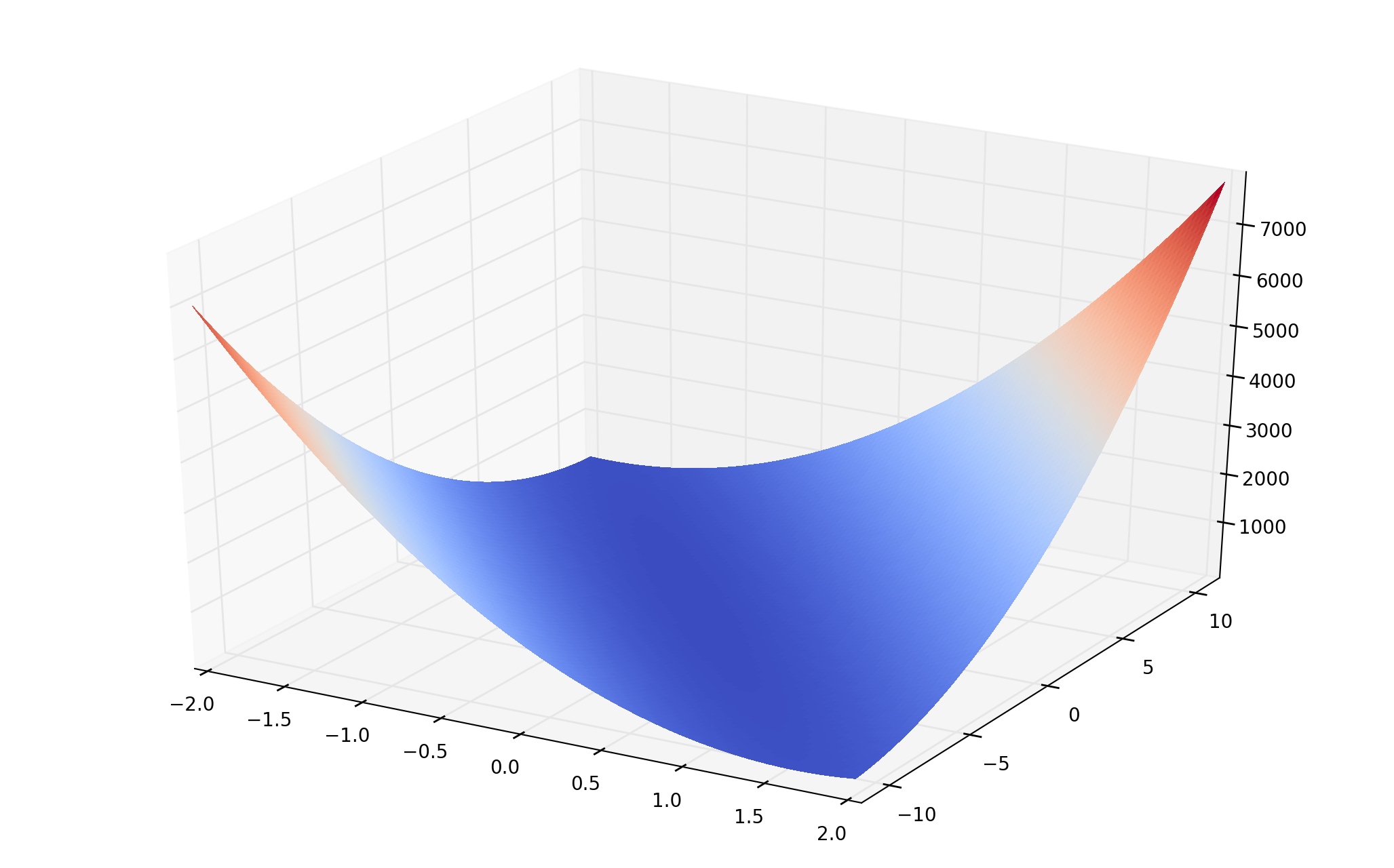
$$\mathcal{L}(\theta|\mathcal{X})\propto -\sum_{t=1}^{n} [y^t - g(x^t|\theta)]^2$$

Max(likelihood) = Min(squared error)

Note: the squared error is often written like this for convenience:

Likelihood

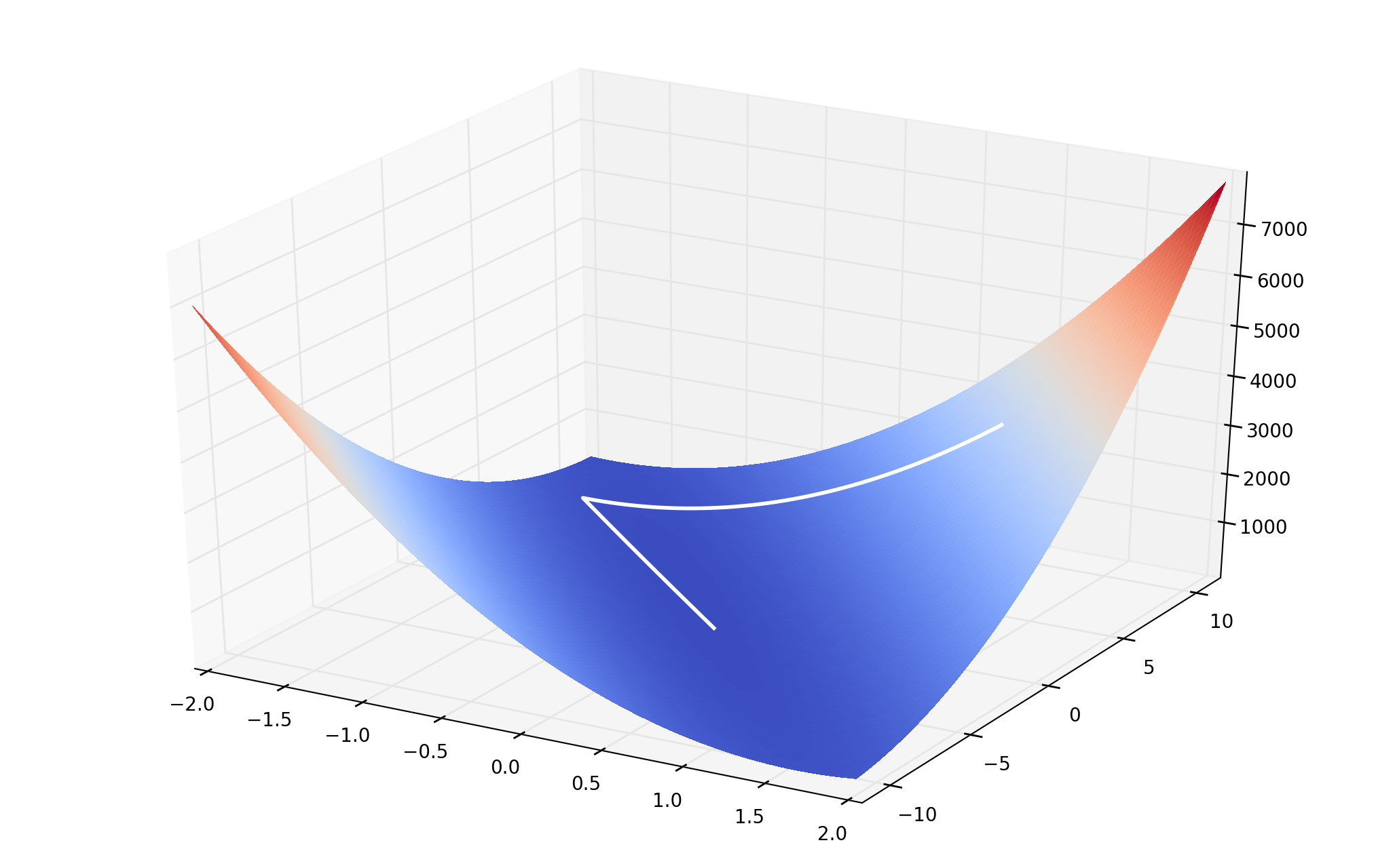
Having the Loss function, we do gradient descent

Likelihood

Having the Loss function, we do gradient descent

Likelihood

Having the Loss function, we do gradient descent

Maximum Likelihood

Finding a loss function by ML

$$\theta_{ML} = \underset{\theta}{\operatorname{arg}\,\operatorname{max}}\;P(Y|X;\theta) = \underset{\theta}{\operatorname{arg}\,\operatorname{max}}\;\sum\limits_{i=1}^{m}\operatorname{log}\,P(y^i|\vec{x}^i;\theta)$$

We want to maximize likelihood
This means minimizing cross entropy between model and data
Loss function depends on the model output:

Regression: linear output, mean squared error
Binary classification: class probability, sigmoid output, logistic loss

(Also for multilabel classification, with probability for each label)

N-ary classification, use softmax and the softmax cross entropy:

Activation, Loss and Optimization

Optimizers

Minimizing the loss function

We want to minimize the loss function (e.g. cross-entropy for ML) to obtain $\theta$ from some data
Numerical optimization is outside the scope of this course

But it's useful to have some knowledge of the optimizers

Optimizers

Minimizing the loss function

So far we saw tf.optimizers.SGD

Basic gradient descent algorithm, single learning rate.
Stochastic gradient descent: use gradient computed at each example, selected at random
Mini-batch gradient descent: updates after computing the total gradient from a batch of randomly selected examples.
Can include momentum (and you should use momentum, in general)

This is just an alias for the tf.keras.optimizers.SGD class

We'll be using Keras explicitely from now on

Optimizers

Minimizing the loss function:

Different parameters may best be changed at different rates

tf.keras.optimizers.Adagrad
Keeps sum of past (squared) gradients for all parameters
Divides learning rate of each parameter by this sum
Parameters with small gradients will have larger learning rates, and vice-versa
Since Adagrad sums previous gradients, learning rates will shrink

(good for convex problems)

Optimizers

Minimizing the loss function:

Some parameters may be left with too large or too small gradients

tf.keras.optimizers.RMSProp
Keeps moving root of the mean of the squared gradients (RMS)
Divides gradient by this moving RMS
Updates will tend to be similar for all parameters.
Since it uses a moving average, learning rates don't shrink

Good for non-convex problems, and often used in recurrent neural networks

Most famous unpublished optimizer

Optimizers

Minimizing the loss function

tf.keras.optimizers.Adam

Adaptive Moment Estimation (Adam)
Momentum and different learning rates using an exponentially decaying average over the previous gradients

tf.keras.optimizers.AdamW

Adaptive Moment Estimation (Adam)
Similar to Adam but with Weight Decay, generalizes better than Adam
Fast to learn but may have convergence problems

How to choose?

There is no solid theoretical foundation for this
So you must choose empirically

Which is just a fancy way of saying try and see what works...

Learning Rate

Choosing the best learning rate

Optimizers can have other parameters, but all have a learning rate
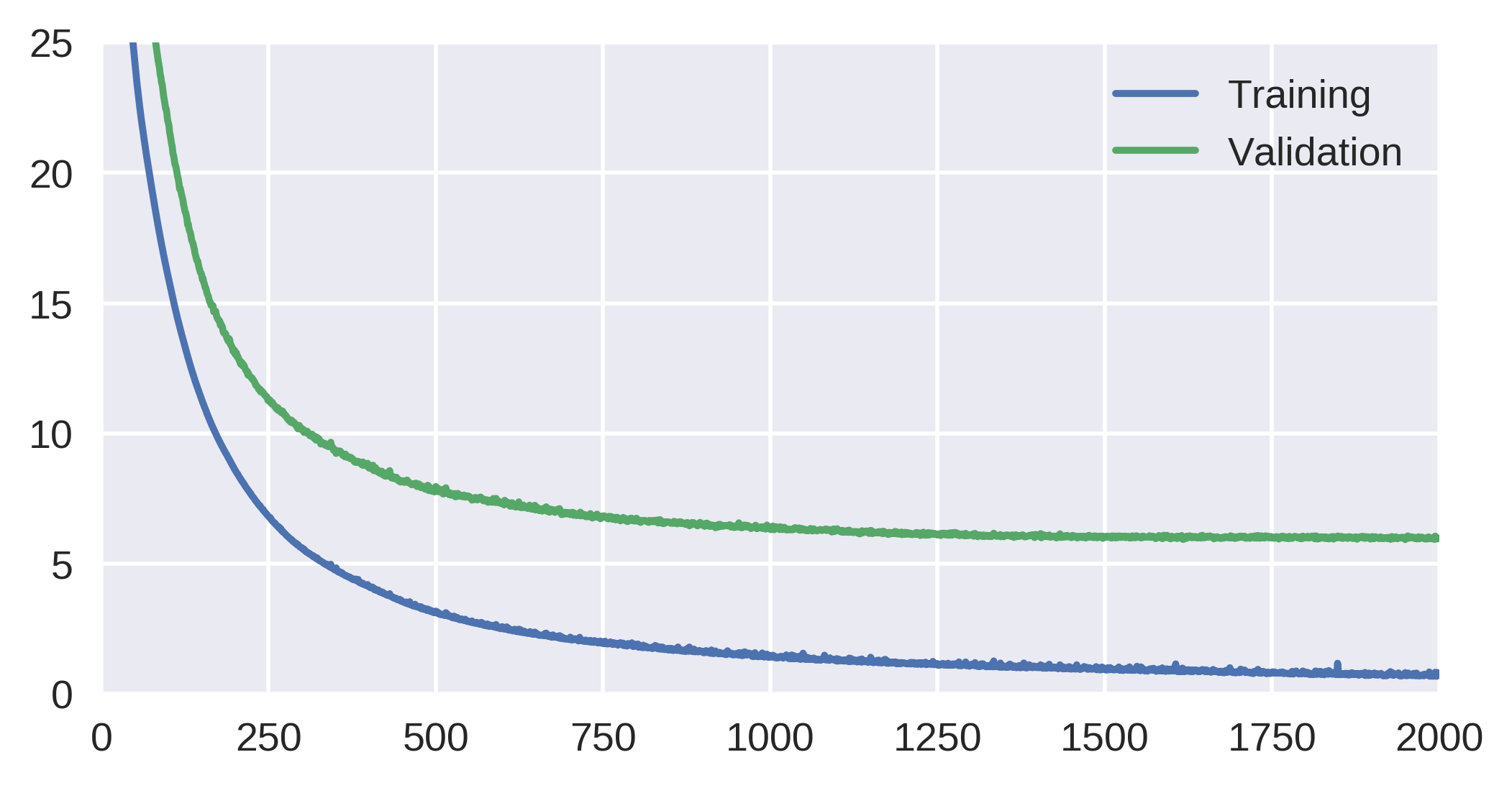
Too high a learning rate can lead to convergence problems

Learning Rate

However, if learning rate is too small training can take too long
Try to make it as high as you can while still converging to low error

(you can experiment with a subset of your training set, even if overfitting)

Batch Normalization

Normalizing (standardizing) activations

Compute running averages and standard deviations during training

And standardize the inputs to each layer

Just like we do for the inputs to the network, do for hidden layers too

Makes learning easier by preventing extreme values
Eliminates shifts in mean and variance during training
Reduces the need for each layer to adapt to the changes in the previous one

This can be done easily in Keras

The mean, standard deviation and rescaling can all be part of backpropagation

AutoDiff takes care of the derivatives

So we can add batch normalization as an additional layer

Activation, Loss and Optimization

Overfitting and Validation

The goal of (supervised) learning is prediction

And we want to predict outside of what we know

Overfitting

The problem of adjusting too much to training data

and losing generalization

Two ways of solving this:

Select the right model: model selection
Adjust training: regularization

Overfitting and Validation

How to check for overfitting

We need to evaluate performance outside the training set

Test set: we need to keep this for final evaluation of error rate

We can use a validation set
Or we can use cross-validation

Overfitting and Validation

How to check for overfitting

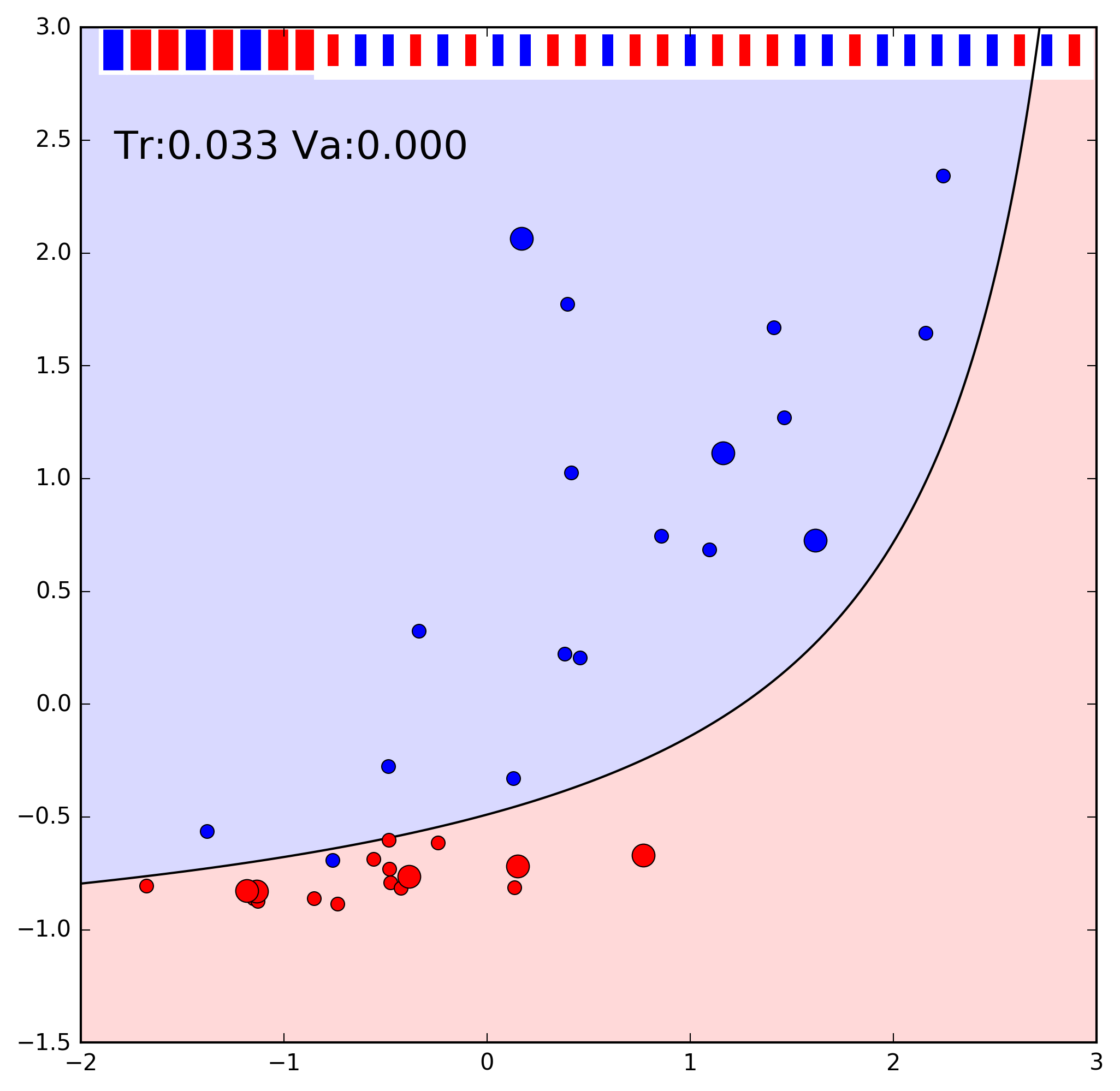
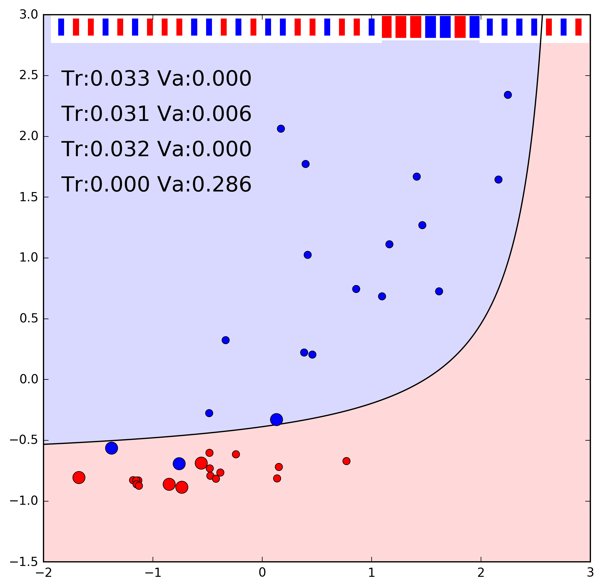
Cross-Validation:

Split training set into K folds, average validations training on the k-1

Overfitting and Validation

How to check for overfitting

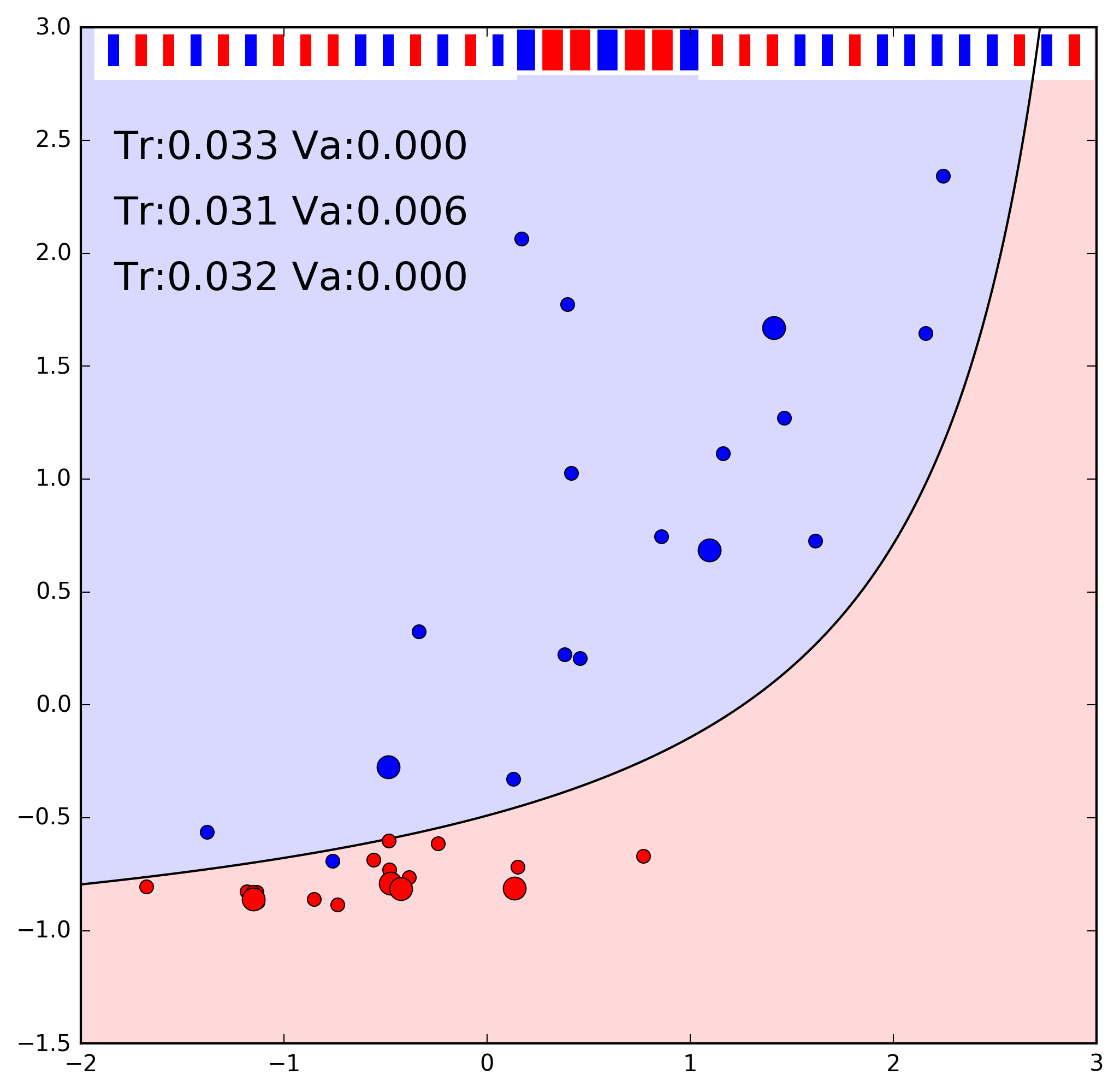
Cross-Validation:

Split training set into K folds, average validations training on the k-1

Overfitting and Validation

How to check for overfitting

Option 1: Cross-validation on training set, test

Good when data is scarcer
Better estimate of true error
More computationally demanding

Option 2: train, validation for preventing overfitting, test

Good when we have lots of data (which is generally the case for DL)

Cross-validation is widely used outside deep learning
With deep learning training and validation is more common

Deep networks take some time to train

Overfitting and Validation

Estimating the true error

True error: the expected error over all possible data

We cannot measure this, since we would need all possible data

Must be estimated with a test set, outside the training set
This cannot be the validation set if the validation set was used to optimize hyperparameters

We choose the combination with the smallest validation error, this makes the estimate biased.

Solution: reserve a test set for final estimate of true error

This set should not be used for any choice or optimization

Overfitting

Model Selection

If the model adapts too much to the data, the training error may be low but the true error high

Example: Auto MPG problem, 100-50-10-1 network.

Overfitting

Model Selection

One way of solving this problem is to use a simpler model (assuming it can fit the data)

Example: Auto MPG problem, 30-10-1 network.

Overfitting

Model Selection

If the model is too simple, then error may become high

(Underfitting)
Example: Auto MPG problem, 3-2-1 network.

Activation, Loss and Optimization

Regularization in ANN

Regularization

Penalizing parameter size

To reduce variance, we can force parameters to remain small by adding a penalty to the objective (cost) function:
Where $\alpha$ is the weight of the regularization

Note: in ANN, generally only the input weights at each neuron are penalized and not the bias weights.

The norm function $\Omega(\theta)$ usually takes these forms:

L$^2$ Regularization (ridge regression): penalize $||\theta||^2$
L$^1$ Regularization: penalize $\sum_i |\theta_i|$

Regularization

L$^2$ Regularization is weight decay

If we penalize $w^2$, the gradient becomes:
This means the update rule for the weight becomes
We decrease the magnitude of $w$ to $(1-\epsilon 2 \alpha)$ per update
This causes weights that do not contribute to reducing the cost function to shrink

Regularization

L$^1$ Regularization

If we penalize $|w|$, the gradient becomes:
This penalizes parameters by a constant value, leading to a sparse solution

Some weights will have an optimal value of 0

L$^1$ vs L$^2$ Regularization

L$^1$ minimizes number of non-zero weights
L$^2$ minimizes overall weight magnitude

Regularization

Dataset augmentation

More data is generally better, although not always readily available
But sometimes we can make more data
E.g. Image classification:

Translate images. Rotate or flip, if appropriate (not for character recognition)

Wang et al, 2019, "A survey of face data augmentation".

Regularization

Dataset augmentation by noise injection

Noise injection is an (implicit) form of dataset augmentation

Add (carefully) noise to inputs, or even to some hidden layers

Noise can also be applied to the weights
Or even the output

There may be errors in labelling
Or for label smoothing: use $\frac{\epsilon}{(k-1)}$ and $1-\epsilon$ instead of 0 and 1 for target
This prevents pushing softmax or sigmoid to infinity

Regularization

Early stopping

Use validation to stop at best point

Constrains weights to be closer to starting distribution

Regularization

Bagging

Training a set of models on different subsets of the data
use the average response (or majority vote)
Improves performance, as it reduces variance without affecting bias, and ANN can have high variance
However, it can be costly to train and use many deep models.

Regularization

Dropout

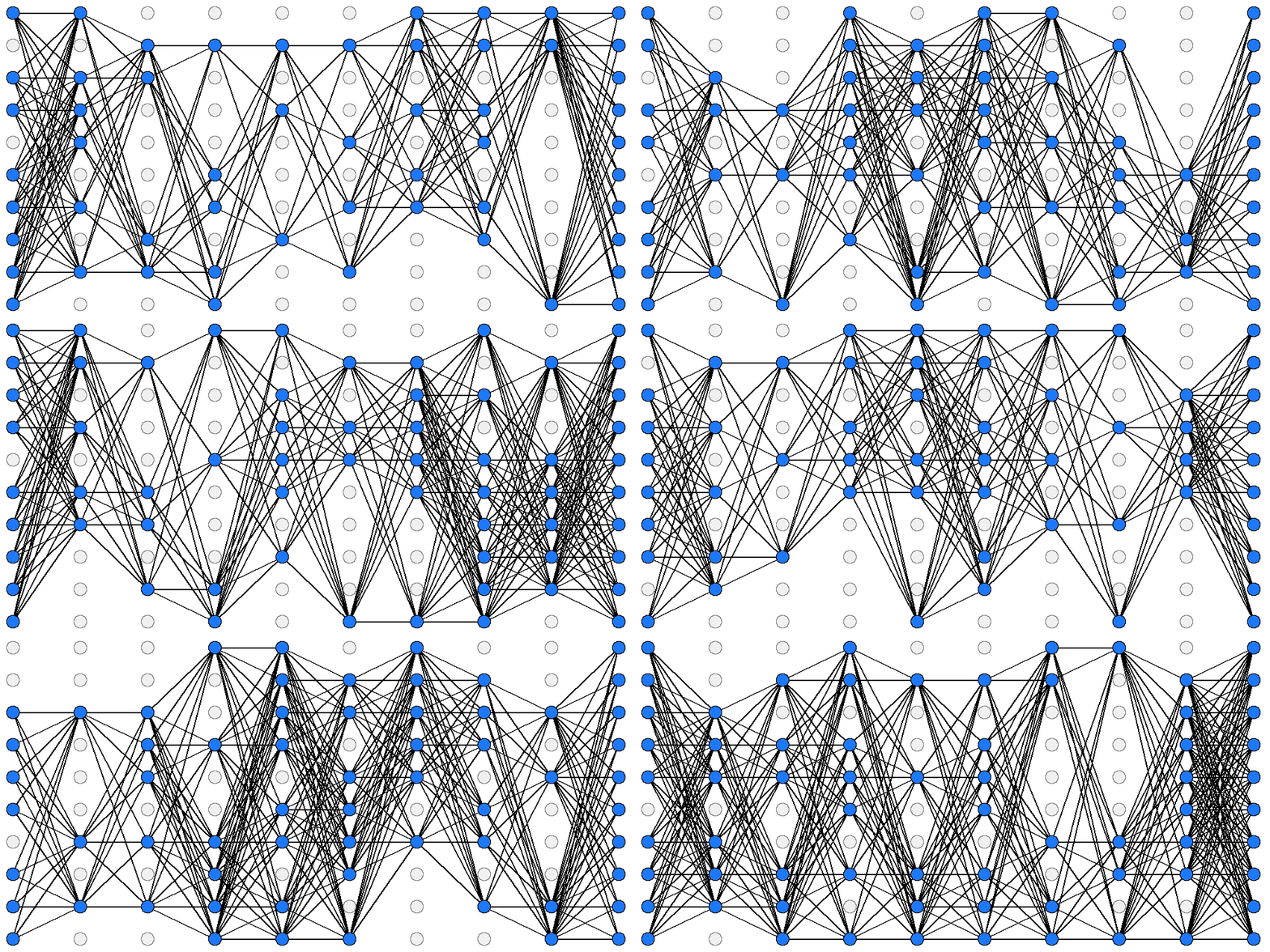
"Turns off" random input and hidden neurons in each minibatch

Regularization

Dropout

Dropout does model averaging implicitely
Turning off neurons at random trains an ensemble of many different networks
After training, weights are scaled by the probability of being "on"

(same expected activation value)

Keras automatically adjust for this when we use a Dropout layer

Activation, Loss and Optimization

Summary

Activation and Loss

Summary

The vanishing gradients problem, ReLU
Activations for hidden and output layers
Loss functions
Optimizers, learning rate, batch normalization
Model selection and Regularization